In-Class_Ex2_EHSA

Getting Started

Installing and Loading R Packages

Loading R packages. The plotly library is added to create interactive maps.

pacman::p_load(sf, sfdep, tmap, plotly, tidyverse, knitr)

The Data

Importing geospatial data

st_read() can be used to read the shape file data set into an R sf data frame

hunan <- st_read(dsn = 'data/geospatial',
                 layer = 'Hunan')

Reading layer `Hunan' from data source 
  `D:\phlong2023\ISSS624\In-Class_Ex\In-Class_Ex2\data\geospatial' 
  using driver `ESRI Shapefile'
Simple feature collection with 88 features and 7 fields
Geometry type: POLYGON
Dimension:     XY
Bounding box:  xmin: 108.7831 ymin: 24.6342 xmax: 114.2544 ymax: 30.12812
Geodetic CRS:  WGS 84

Importing time series file

read_csv() can be used to read the time series file into an R data frame

GDPPC <- read_csv('data/aspatial/Hunan_GDPPC.csv')

Creating a Time Series

spacetime() can be used to create a Space Time Cube

GDPPC_st <- spacetime(GDPPC, hunan,
                      .loc_col = 'County',
                      .time_col = 'Year')

is_spacetime_cube() can be used to check whether the created object is actually a spacetime cube

is_spacetime_cube(GDPPC_st)

[1] TRUE

Creating Inverse Distance Weight Matrix Columns for GI*

GDPPC_nb <- GDPPC_st %>%
  activate('geometry') %>%
  mutate(nb = include_self(st_contiguity(geometry)),
         wt = st_inverse_distance(nb, geometry,
                                  scale = 1,
                                  alpha = 1),
         .before = 1)%>%
  set_nbs('nb') %>%
  set_wts('wt')

Computing GI*

Computing GI* using the newly created data frame with the neighbor list and weight matrix for each county for each year

gi_stars <- GDPPC_nb %>%
  group_by(Year) %>%
  mutate(gi_star = local_gstar_perm(GDPPC, nb, wt)) %>%
  unnest(gi_star)

Man-Kendall Test

Performing Emerging Hotspot Analysis

emerging_hotspot_analysis() can be used to perform the Emerging Hotspot Analysis using the space time cube object

ehsa <- emerging_hotspot_analysis(
  x = GDPPC_st,
  .var = 'GDPPC',
  k = 1, #Comparing the Time Series sequentially (e.g. 2012 vs 2013)
  nsim = 99
)

Plotting the distribution of hotspot type

ggplot(ehsa, aes(x=classification))+
  geom_bar()+
  theme_classic()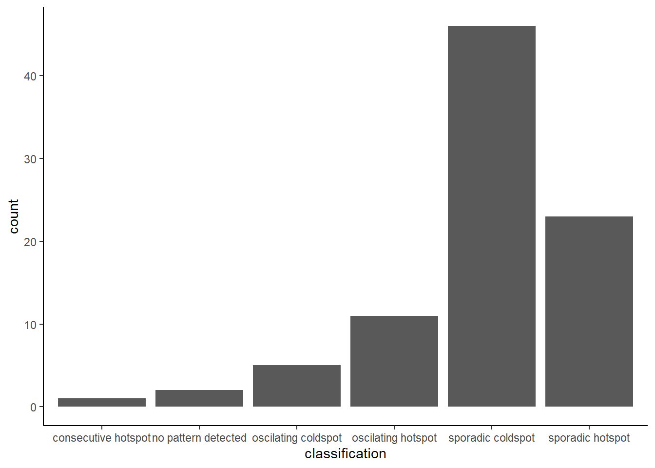

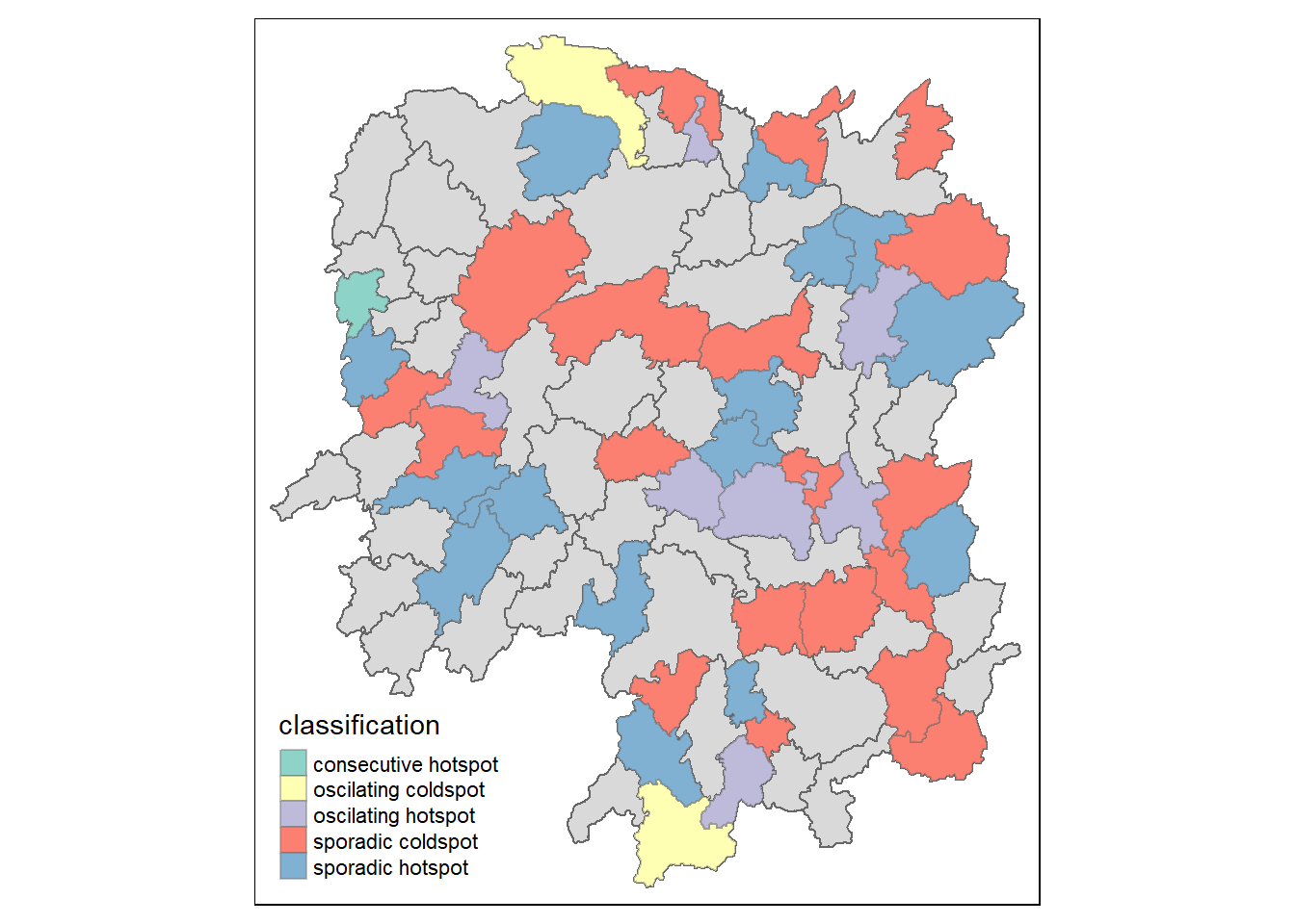
Visualizing EHSA

ehsa_rename <- ehsa %>%
  rename(County = location)

hunan_ehsa <- left_join(hunan, ehsa_rename,
                        by = 'County')

ehsa_sig <- hunan_ehsa %>%
  filter(p_value < 0.05)
tmap_mode('plot')
tm_shape(hunan_ehsa) +
  tm_polygons()+
  tm_borders(alpha = 0.5)+
  tm_shape(ehsa_sig)+
  tm_fill('classification')+
  tm_borders(alpha = 0.4)